The INSIGHT Health Data Research Hub is an NHS-led initiative that makes large datasets of routinely collected eye data available for research. Softwire have been working with Moorfields Eye Hospital, the lead NHS trust for INSIGHT, for a number of years. As part of this work, we regularly create large datasets of images, often tens of TB each. These datasets have enabled groundbreaking research, such as on the detection of early signs of Alzheimer’s disease and Parkinson’s disease.
When creating these large datasets, it’s not unusual to need to modify every single image to update a piece of metadata, for example to include specific anonymised clinical metadata. Google Cloud Platform (GCP) Dataflow is perfect for these sorts of embarrassingly parallel jobs – jobs that are simple to split into parallel tasks.
Like all specialised tools there are trade-offs and a few gotchas to be aware of.
What is Dataflow?
Dataflow is built on top of Apache Beam which provides, to quote their documentation – “an open source, unified model for defining both batch and streaming pipelines”. It supports a variety of languages and execution frameworks such as Kotlin, Spark and Flink – but we happen to be using Python and Google Dataflow, a GCP-managed execution framework.
What does all this mean in practice, though? You, the programmer, describe the data processing to be done in the Beam language of Pipelines, PTransforms, and PCollections, and then Dataflow will handle running your pipeline, including:
- Scalability: Creating more workers as required and dynamically rebalancing work across them.
- Work-balancing: Splitting up the work into batches, balancing it across workers, and serialising and de-serialising the results of individual stages so they can be passed between workers.
- Fault-tolerance: Each individual transform will be retried up to four times before the whole pipeline is failed (in batch mode that is, streaming mode is more complicated).
Beam also comes with a huge array of built-in connectors for upstream and downstream systems, such as filesystems and databases. These are called ‘Sources’ and ‘Sinks’ in Beam language. So, if you need to load data from a common data source such as GCS or a Postgres database, or write to a common sink like BigQuery, it’s very straightforward.
On the other hand, Beam provides few primitives to make sure that your data is processed in any specific order or how quickly it is processed, and you can forget about most shared state. This makes Beam extremely well suited for streaming data analytics and easily parallelisable workloads such as running ML models, but a poor choice for most stateful or low-latency workloads.
Lessons Learned
As with all specialised tools, you need to know the problems it’s suited for and those it isn’t, to design your code according to Beam’s patterns, and to understand its pitfalls.
1) Think in Pipelines, PTransforms and PCollections
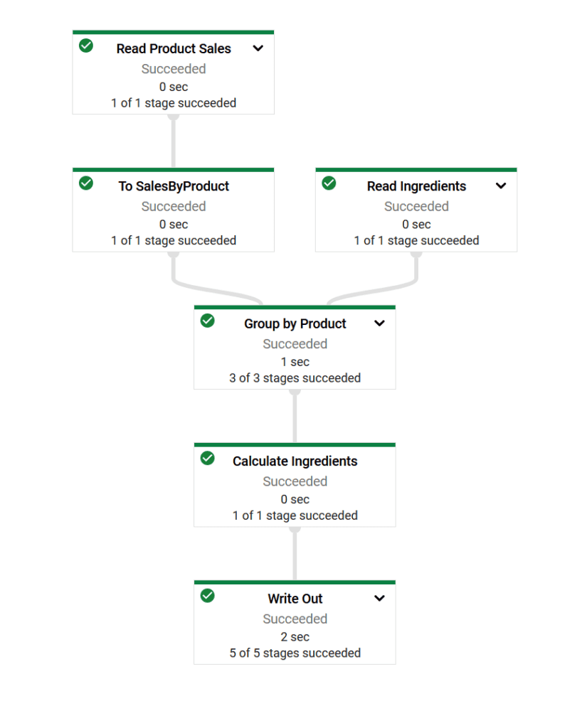
A picture is worth a thousand complex technical definitions:

A simple pipeline showing some data sources, a CoGroupByKey aggregation (we’ll get to these later), some regular PTransforms, and a data sink. This visualisation is generated automatically by GCP and allows you to click through into component PTransforms as well as showing live metrics while running the pipeline. The full source code is available here: https://github.com/Softwire/ExampleDataflowPipeline
Writing your data pipelines for Beam requires a bit of a step change in how you think – you need to think in terms of Beam primitives like PCollections, a set or stream of data, and PTransforms, the data processing steps that transform one PCollection into another. The one that takes the most getting used to however is aggregation. The primary aggregation pattern in Beam is similar to MapReduce: group all elements by a key and combine the elements.
This is a different way of thinking if you are used to SQL constructs like INNER JOIN and OUTER JOIN. Let’s say you have two datasets, tracking, I don’t know, sensor readings for temperate SENSOR_TEMP and sensor readings for humidity SENSOR_HUMID, and you need to combine them by the SENSOR_ID to do some processing. You can’t simply SELECT … FROM SENSOR_TEMP JOIN SENSOR_HUMID ON (SENSOR_ID). Instead, you would CoGroupByKey using the SENSOR_ID to collect all the elements with the same SENSOR_ID together before downstream processing.
2) Make all transforms idempotent
Beam promises to deliver each message to downstream storage, but it does not promise to only process each message once. If you step back for a minute, this is quite obviously not something it could promise; if a worker became unresponsive after an element was processed, Dataflow would have no choice but to retry the element, causing any side effects to be run twice. Beam actually takes this a lot further: it groups elements into a bundle, and if one element in a bundle fails, then all bundle elements will be retried. Thus, you can expect elements to be retried often, even if they themselves didn’t fail.
Hence, if you write a custom integration for an upstream or downstream system, you need to write it with this in mind: all transforms must be idempotent because they might be tried multiple times.
On one INSIGHT workload involving the processing of larger than usual amounts of imaging data, spikes in memory usage would cause the Dataflow workers to run out of memory. This would happen after some elements had been written to storage, and upon retrying would attempt to write the same file again. Of course, we’ve written our pipelines to be idempotent, and we skip the file write the second time around if we see it’s already present.
3) Reshuffle to break pipeline fusion
If you’ve ever run workloads on Apache Hadoop or similar systems, you’ll be familiar with sharding the input in advance. Take a simple example – you want to copy a batch of files. You might shard using the input filenames, so those beginning with A are processed on the first worker, those beginning with “B” on the second, and so on. The problem is that, even with clever heuristics, it’s often impossible to know up-front how long each shard will take to process. For example some files might be much bigger than others, and inevitably there are stragglers – shards that are still processing long after the others have completed.
In Dataflow, work is instead rebalanced dynamically across workers: a worker with too much will assign it to other idle workers. Dataflow calls this ‘liquid sharding’ or ‘dynamic rebalancing’. However, there are some situations where you still do need to worry about how work is balanced.
This is because behind the scenes, Beam performs more optimisations on pipeline creation than the batching of elements we talked about earlier. For example, if one transformation step outputs a bunch of elements that are immediately fed into another transformation, the two transforms may be fused together into a single “stage”. This is often more efficient as it avoids the I/O involved in transferring data between stages.
But what happens if the first of the two fused transforms outputs millions of times more elements than it receives (a high “fanout”)? Such a situation is common in sources that query upstream systems. This can introduce a performance bottleneck: if the first transform only has 10 elements, then the whole fused stage can also only be split across at most 10 workers.
This kind of fusion can be particularly frustrating, as your pipeline will run, but only very slowly, and without scaling up as you think it should. In our INSIGHT pipelines we have a couple of RDBMS data sources that needed the addition of a step to break this pipeline fusion.
4) Watch out for hot keys
Here’s another example of where you do need to pay attention to how work is balanced. Remember the aggregation example from earlier with the sensors with CoGroupByKey? The CoGroupByKey primitive takes a list of key-value pairs and groups them by the key. If you have a ‘hot key’ – a key that has a very large number of values, much more than your other keys – then you may find that your pipeline stalls with one worker very busy while all of the others sit idle. This is because CoGroupByKey will perform all of the aggregation for a given key on one worker.
One easy solution for this is to avoid hot keys altogether! But in case that isn’t possible, there are some methods that will fan out the hot key, such as with_hotkey_fanout – this will fan out the aggregation step to be run in parallel.
On INSIGHT, we often need to link various types of imaging and clinical metadata, and hot keys can easily occur if a mistake is made in the key we are using for linkage. To oversimplify, if you find a patient who has had one million Optical Coherence Tomography (OCT) scan images, you probably have other problems than just a hot key!
Summary
Dataflow is a very powerful tool for certain types of large dataset processing, but due to its architecture it does have some quirks that you need to be aware of.
Many of these will manifest as either sporadic and unusual errors, such as failing to make your transforms idempotent, or poor performance, such as incorrect management of hot keys.
Dataflow also comes with good built-in monitoring tooling, including the recent addition of Cloud Profiler, essentially for catching these kinds of issues if they slip through the net of code review.
Want to find out more about our data engineering services? Get in touch to tell us about your project.


